
Predicting Low Birth Weight Using Statistical Modeling
1. Introduction
Low-birth-weight newborns have significantly higher infant death rates. Various maternal factors during pregnancy can significantly influence the likelihood of carrying a pregnancy to term and, consequently, delivering a neonate with a low birth weight. To improve prenatal care and reduce unfavorable delivery outcomes, it is essential to identify these risk factors.
This study utilizes data from 134 births recorded at Baystate Medical Center in Springfield, Massachusetts. The dataset includes an indicator for low birth weight as the primary response variable, alongside multiple maternal characteristics and risk factors associated with birth outcomes. Additionally, the dataset contains actual birth weights, enabling a comprehensive analysis of the predictors influencing low birth weight.
Variables Measured:
low: Indicator of birth weight less than 2.5kg.
age: Mother’s age in years.
lwt: Mother’s weight in pounds at last menstrual period.
race: Mother’s race (white, black, other).
smoke: Smoking status during pregnancy (yes/no).
ht: History of hypertension (yes/no).
ui: Presence of uterine irritability (yes/no).
ftv: Number of physician visits during the first trimester.
ptl: Number of previous premature labors. (in this data its 0 or 1)
bwt: Birth weight in grams.
2. preliminary exploratory analysis
From looking at the data we can see that the binary variable “low” (0 or 1) has the mean of 0.3358, suggesting that approximately 33.6% of births in the dataset fall into this category. Maternal age ranges from 14 to 45 years, with a median of 22 years, while the mother’s weight in pounds at last menstrual period (lwt) varies between 85 and 250 pounds, with a median of 120.5 pounds. Additionally, both maternal age and mother’s weight (lwt) exhibit right-skewed distributions (Figure 1), indicating that most mothers in the dataset are younger and have lower weights, with fewer observations extending toward higher values. The dataset also includes categorical variables such as race (Black: 18, White: 67, Other: 49), smoking status (79 non-smokers, 55 smokers), and medical risk factors such as hypertension history (ht), where 125 individuals do not have it and 9 have it, and uterine irritability (ui), where 116 individuals do not have it and 18 have it. Additionally, birth weight (bwt) ranges from 709 to 4990 grams, with a median of 2984 grams and mean of 2914 grams.
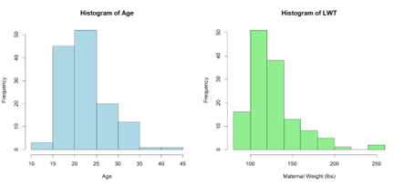
Figure 1
Based on the Figure 2, we can observe potential influences of different factors on birth weight (bwt). Some variables show more pronounced differences between groups, indicating a stronger potential impact on birth weight. Notably, ht (history of hypertension) appears to have a significant effect, as infants born to mothers with hypertension (ht = 1) tend to have lower birth weights compared to those without hypertension. Smoking status (Smoke) also suggests a possible influence, where mothers who smoked during pregnancy (Smoke = 1) seem to have slightly lower birth weights on average compared to non-smokers. Race exhibits some variation, with differences among black, white, and other categories, though the differences are less pronounced. ui (uterine irritability) and ptl (preterm labor history) might also contribute to lower birth weights, as indicated by a downward shift in the median and interquartile range for ui = 1 and ptl = 1. The ftv (number of physician visits during pregnancy) boxplot does not show a strong effect, suggesting that this factor alone might not be a major determinant of birth weight. Overall, factors like ht, smoke, ui, and ptl could show the strongest signs of being associated with low birth weight.
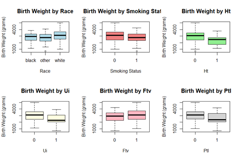
Figure 2
Now, we will examine the correlations among continuous variables to identify potential relationships and assess their significance in the analysis. Figure 3 provides a visual representation of the relationships between key continuous and categorical variables in the dataset, including age, maternal weight at the last menstrual period in pounds (lwt), previous preterm labor (ptl), birth weight in grams (bwt), and smoking status (smoke). Each scatterplot displays the distribution and potential correlations between pairs of variables.
From figure 3, we observe that lwt and bwt appear to have a positive correlation, meaning that lower maternal weight may be associated with lower birth weight. Additionally, the age variable is widely distributed without a clear linear trend with other continuous variables, indicating weaker collinearity.
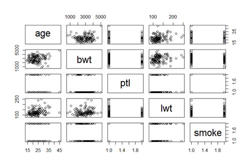
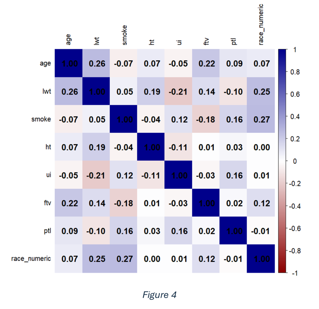
Figure 4 presents a heatmap illustrating the correlations between all numeric variables in the dataset. The intensity of the colours indicates the strength and direction of the relationships, with darker shades representing stronger correlations. Overall, most variables exhibit weak correlations, suggesting minimal collinearity among predictors.
Note that the outcome variable low is essentially a dichotomized representation of the bwt variable; therefore, bwt is excluded from further analyses. In addition, we want to check for confounding in our study on low birth weight (low) to ensure that the relationships between the independent variables and low are not distorted by a third variable. Confounding occurs when a variable is associated with both the predictor and the outcome, leading to misleading conclusions if not properly adjusted for.
Table 1
| Univariate | Multivariate | ||
Variable | OR | CI | OR | CI |
Age | 0.969 | (0.90,1.04) | 0.97 | (0.89,1.06) |
Lwt | 0.99 | (0.979,1.01) | 0.99 | (0.98,1.01) |
Ptl1 | 4.44 | (1.76,11.23) | 3.54 | (1.25,10.05) |
Smoke1 | 1.62 | (0.79,3.35) | 2.1 | (0.82,5.55) |
Race other | 1.18 | (0.39,3.55) | 1.36 | (0.38,4.8) |
Race white | 0.53 | (0.18,1.60) | 0.43 | (0.12,1.49) |
Ht1 | 4.41 | (1.05,18.56) | 6.43 | (1.32,31.32) |
Ui1 | 2.89 | (1.05,7.95) | 3.12 | (0.97,9.99) |
Ftv1 | 0.71 | (0.34,1.48) | 0.98 | (0.41,2.34) |
In our dataset, Table 1 suggests potential signs of confounding with the variables ht, and smoke. The differences observed between the univariate and multivariate odds ratios indicate that these factors may be influencing the relationships between other variables in the analysis.
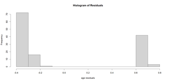
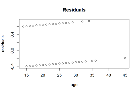
If we apply the linear regression model, although the dependent variable is not continuous, we find out that the residuals histogram (Figure 5) is not normally distributed. Additionally, the variance is not constant, indicating a lack of homoscedasticity (Figure 6). These findings suggest that the assumptions of linear regression may not hold, requiring alternative modeling approaches.
3. The appropriate Generalized Linear Model (GLIM)
In our dataset the response variable “low” which is an indicator of birth weight is dichotomous, this term refers to a variable that can only take on two possible values or categories. This variable is coded as 0 if the birth weight is less than or equal 2.5 kg and 1 if it exceeds this threshold.
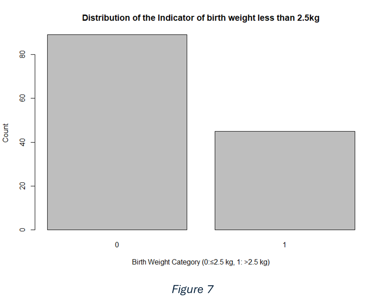
As we saw earlier the response residuals does not distribute as normal. So, in this case we decided to use one of the Generalized Linear Models (GLMs) that accommodates non-normal response distributions. For this case the response variable is distributed as a binomial distribution as shown in (figure 7). So, we will use logistic regression, which is a type of GLM, specifically designed for this.
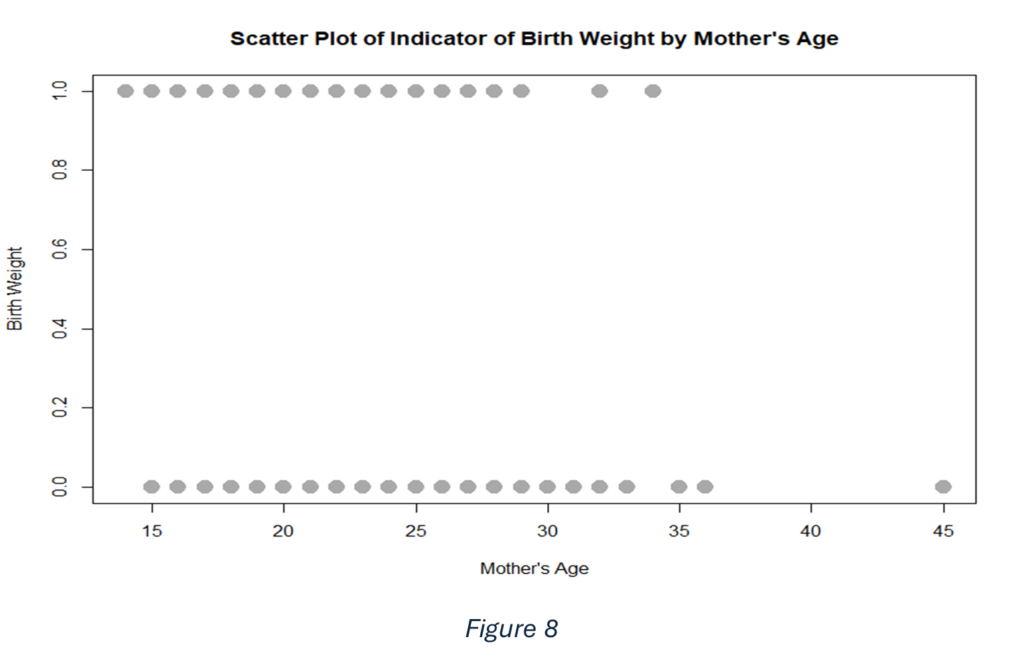
It could be that the mother’s age affects the birth weight of the newborn. On the horizontal axis of figure 8 is the mother’s age, and on its vertical axis is the binary indicator of birth weight. Because the birth weight is dichotomous, the points form two parallel lines rather than being spread continuously up the y-axis. Although the figure clearly shows which observations fall into each birth weight category at various ages, it provides only a limited view of how mother’s age may influence birth weight. This plot suggests that there is no clear pattern indicating that the mother’s age strongly affects birth weight. Both birth weight outcomes appear across similar age ranges, indicating that age alone does not seem to distinguish between the two categories. A key challenge with this scatter plot is that the outcome takes only two values (0 or 1). There is considerable variability: mothers of similar ages can have either birth weight category, or no clear trend emerges simply from looking at the raw scatter of points.
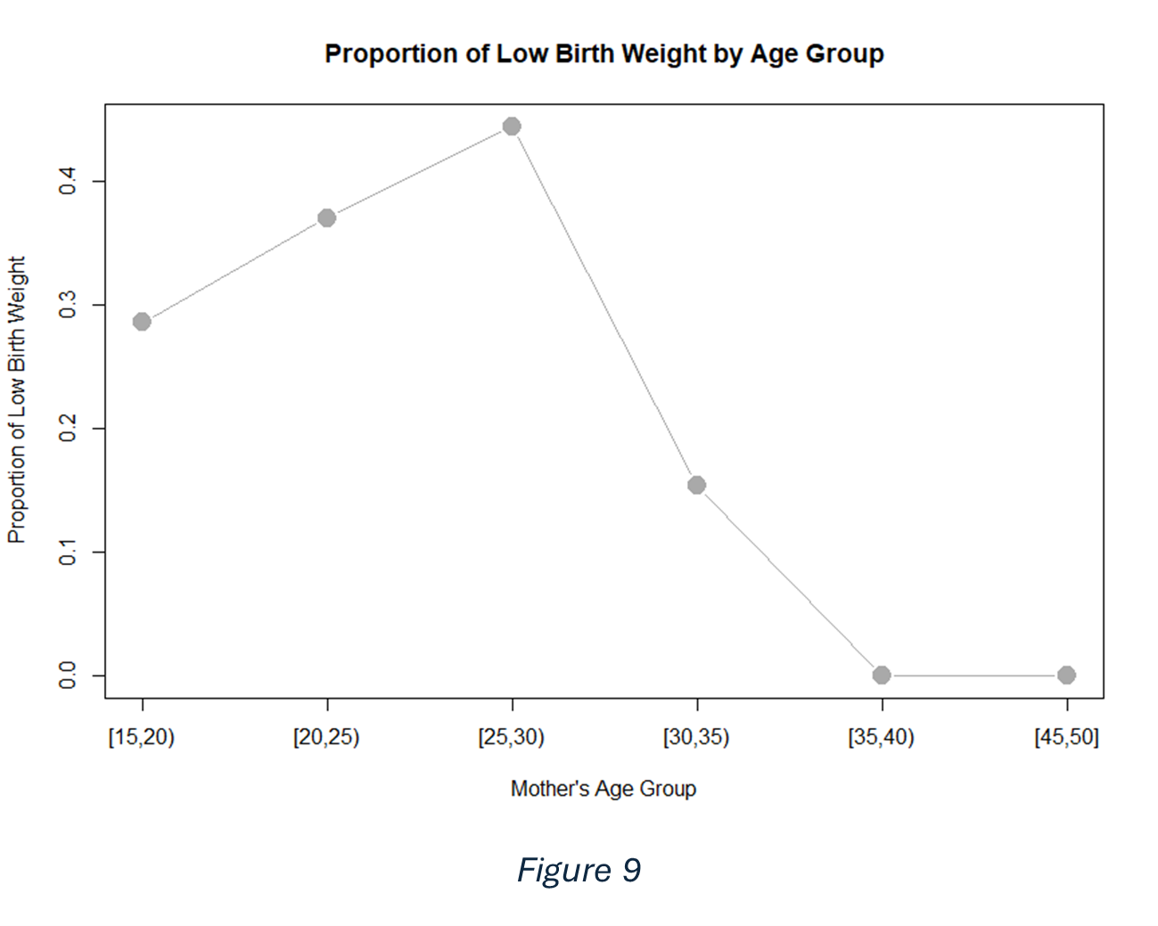
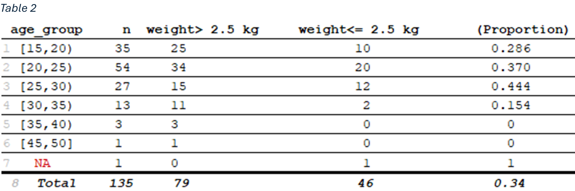
One common way to address this issue is to group the mother’s age into intervals (for instance, 5-year age) and then calculate the proportion of babies in each interval who fall below the threshold for “low” birth weight. Figure 9 and table 2 suggest a non-linear relationship between mother age and the proportion of low birth weight. Early on, as age increases, the proportion of low birth weight rises, reaching its highest point around the late twenties. After age 30, however, the trend reverses, and the proportion of low-birth-weight declines. This pattern indicates that mother’s age may influence birth weight in a more complex way than a simple linear increase or decrease.
However, a functional form for this relationship still needs to be specified. Grouping and averaging data in this way resembles what we might see if we performed a regression analysis. Yet there are key differences. In any regression setting, the primary quantity of interest is the conditional mean of the outcome given a particular value of the explanatory variable, denoted as E(Y∣x). In the case of a binary outcome like low birth weight, E(Y∣x) is interpreted as the probability that Y=1 (i.e., the baby is low birth weight) given independent variables.
4. Fitting the model (logistic regression)
Logistic regression is a statistical method used to model the relationship between a categorical outcome variable and one or more independent variables. Unlike linear regression, which is used when the outcome variable is continuous, logistic regression is specifically designed for binary or dichotomous outcomes. The goal is to find the best-fitting and most simple model that describes the relationship between the outcome and predictor variables. Hypothesis testing, including likelihood ratio tests, Wald tests, and score tests, are used to determine the significance of independent variables. Goodness-of-fit tests, such as the Hosmer-Lemeshow test and chi-square tests, are employed to assess the adequacy of the model.
By utilized the stepAIC algorithm, a stepwise model selection method that optimizes statistical models by minimizing Akaike’s Information Criterion (AIC). AIC is a widely used measure that evaluates the trade-off between model fit and complexity, defined as:
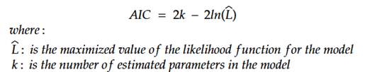
By systematically comparing different predictor subsets, step AIC seeks the model with the lowest AIC, ensuring an optimal balance between goodness-of-fit and simplicity. The algorithm operates iteratively, using both method of the algorithm which combines forward selection with backward elimination to refine the model. At each step, the predictor that leads to the greatest reduction in AIC is either included or excluded, stopping when no further improvement is possible. Resulting in using the following model:
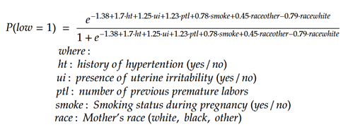
The coefficients that we get as a result of applying the logistic regression are shown in table3. As shown in it all the variables are dichotomous independent variables, so the coefficient represents the change in the log-odds of the outcome for a one-unit change in the predictor, where the predictors can only take two values (0 or 1), the odds ratio approximates how much more likely the outcome is to be present when x = 1 compared to when x = 0.
Table 3
Coefficients: | Estimate | Std. Error | Z value | Pr(>|z|) |
(Intercept) | -1.38 | 0.58 | -2.36 | 0.018* |
ht | 1.7 | 0.78 | 2.17 | 0.03* |
ui | 1.25 | 0.58 | 2.15 | 0.03* |
ptl | 1.23 | 0.51 | 2.41 | 0.016* |
smoke | 0.78 | 0.46 | 1.67 | 0.095. |
Race other | 0.45 | 0.62 | 0.72 | 0.47 |
Race white | -0.79 | 0.62 | -1.28 | 0.20 |
In this case, the likelihood of an infant being born with low birth weight is influenced by various variables. Specifically, if the mother has hypertension, the odds of delivering a low-birth-weight infant increase by a factor of 5.5. Similarly, the presence of uterine irritability results in a likelihood ratio of 3.5, indicating a negligible or slightly reduced risk. A history of premature labor is associated with a 3.4 times lower likelihood of low birth weight. Moreover, if a mother exhibits multiple risk factors—such as hypertension, uterine irritability, and premature labor—the combined effect results in an increased likelihood ratio of \( \frac{e^{-1.38+1.7+1.25+1.23}} {e^{-1.38+1.7(0)+1.25(0)+1.23(0)}} = 65.4 \), highlighting a significant cumulative risk.
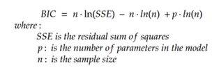
Using Wald’s test, we found that ptl, ht and ui are significant, but the other are not. Although this model is the best model according to the AIC, but it has the variable ht which we have a little doubt that it has confounding. So, we will also find a model using the BIC which is Bayesian Information Criterion -a criterion used for model selection. It helps to find the best model among a set of possible models. The BIC is calculated as:
The BIC selected 19 different models; the 5 best one was as in table4.
Table 4
| P!=0 | EV | SD | Model 1 | Model 2 | Model 3 | Model 4 | Model 5 |
Intercept | 100 | -0.81 | 0.67 | -0.98 | -1.09 | -1.24 | -1.09 | 0.12 |
Age | 12.8 | -0.01 | 0.02 | . | . | . | . | -0.05 |
Lwt | 8.6 | -0.0007 | 0.003 | . | . | . | . | . |
Smoke | 5.4 | 0.02 | 0.012 | . | . | . | . | . |
ptl | 95.6 | 1.42 | 0.56 | 1.49 | 1.5 | 1.41 | 1.4 | 1.58 |
Ht | 50.2 | 0.82 | 0.98 | . | 1.53 | 1.69 | . | . |
Ui | 25.6 | 0.25 | 0.51 | . | . | 1.04 | 0.89 | . |
Ftv | 7.9 | -0.03 | 0.16 | . | . | . | . | . |
Race other | 0 | 0 | 0 | . | . | . | . | . |
Race white | 0 | 0 | 0 | . | . | . | . | . |
nVar |
|
|
| 1 | 2 | 3 | 2 | 2 |
BIC |
|
|
| -485.85 | -485.32 | -483.99 | -483.63 | -482.55 |
Post prob |
|
|
| 0.245 | 0.187 | 0.097 | 0.081 | 0.047 |
If we examine the probability of a coefficient being included in the model, we find that ptl has a 95.6% probability of not equal 0. Additionally, the intercept is present in the model with the lowest BIC. In addition, the table 5 shows that the coefficient of ptl is statistically significant. Based on these criteria, Model 1 is identified as the optimal choice. As shown in the following equation.
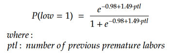
Table 5
coefficients | Estimate | Std. | Z | Pr(>|z|) |
(Intercept) | -0.9808 | 0.2141 | -4.581 | 4.62e-06 *** |
ptl | 1.4917 | 0.4729 | 3.154 | 0.00161 |
In this case, the likelihood of an infant
being born with low birth weight increases by 4.44 times if the mother has a history of previous premature labors, with the confident interval (1.76,11.23). With confident interval of the intercept (-1.4, -0.56) and for the ptl
coefficient its (0.56, 2.42). Using Wald’s test, we found that the p-values of the coefficient is 0.0016 which is significant. Using the
likelihood ratio test between the AIC and BIC models we found out that the residual deviance is changed by 15.1 which was significant, meaning removing the variables ui, ht, smoke and race would reduce the decreases the
predictivity power of the model.